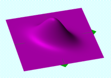
 中心为 (0, 0) 的一个二元高斯概率密度函数,协方差矩阵为 [ 1.00, 0.50 ; 0.50, 1.00 ]。
 一个左下右上方向标准差为 3,正交方向标准差为 1 的多元高斯分布的样本点。由于 x 和 y 分量共变(即相关),x 与 y 的方差不能完全描述该分布;箭头的方向对应的协方差矩阵的特征向量,其长度为特征值的平方根。
在统计学与概率论中,协方差矩阵(covariance matrix)是一个方阵,代表着任两列随机变量间的协方差,是协方差的直接推广。
定义 —
设  是概率空间,
  与
与  是定义在
是定义在  上的两列实数随机变量序列
若二者对应的期望分别为:


则这两列随机变量间的协方差矩阵为:
![{\displaystyle \operatorname {\mathbf {cov} } (X,Y):={\left[\,\operatorname {cov} (x_{i},y_{j})\,\right]}_{m\times n}={{\bigg [}\,\operatorname {E} [(x_{i}-\mu _{i})(y_{j}-\nu _{j})]\,{\bigg ]}}_{m\times n}}](https://wikimedia.org/api/rest_v1/media/math/render/svg/a5156794b781f959d02adb93d3b439bfb543fdf3)
将之以矩形表示的话就是:

![{\displaystyle ={\begin{bmatrix}\mathrm {E} [(x_{1}-\mu _{1})(y_{1}-\nu _{1})]&\mathrm {E} [(x_{1}-\mu _{1})(y_{2}-\nu _{2})]&\cdots &\mathrm {E} [(x_{1}-\mu _{1})(y_{n}-\nu _{n})]\\\mathrm {E} [(x_{2}-\mu _{2})(y_{1}-\nu _{1})]&\mathrm {E} [(x_{2}-\mu _{2})(y_{2}-\nu _{2})]&\cdots &\mathrm {E} [(x_{2}-\mu _{2})(y_{n}-\nu _{n})]\\\vdots &\vdots &\ddots &\vdots \\\mathrm {E} [(x_{m}-\mu _{m})(y_{1}-\nu _{1})]&\mathrm {E} [(x_{m}-\mu _{m})(y_{2}-\nu _{2})]&\cdots &\mathrm {E} [(x_{m}-\mu _{m})(y_{n}-\nu _{n})]\end{bmatrix}}}](https://wikimedia.org/api/rest_v1/media/math/render/svg/7e9a5a14766d082923ed9e794213088c3c32d7ac)
根据测度积分的线性性质,协方差矩阵还可以进一步化简为:
![{\displaystyle \operatorname {\mathbf {cov} } (X,Y)={\left[\,\operatorname {E} (x_{i}y_{j})-\mu _{i}\nu _{j}\,\right]}_{n\times n}}](https://wikimedia.org/api/rest_v1/media/math/render/svg/a813988c7371dfa7dedb84fdaaf86a286bf02b38)
以上定义所述的随机变量序列  和
和  ,也可分别以用行向量
 ![{\displaystyle \mathbf {X} :={\left[x_{i}\right]}_{m}}](https://wikimedia.org/api/rest_v1/media/math/render/svg/96aafe9bf2396bad8aeb8cd26bb9238d30980f79) 与
与 ![{\displaystyle \mathbf {Y} :={\left[y_{j}\right]}_{n}}](https://wikimedia.org/api/rest_v1/media/math/render/svg/bc7061e7cbd2f5e2b0b5dec6628b26ca0ebcabe2) 表示,换句话说:
表示,换句话说:


这样的话,对于  个定义在 上的随机变量
  所组成的矩阵
 ![{\displaystyle \mathbf {A} ={\left[\,a_{ij}\,\right]}_{m\times n}}](https://wikimedia.org/api/rest_v1/media/math/render/svg/d523a9b473aa9f1703fb22dcd25a3a707d80fb9b) , 定义:
, 定义:
![{\displaystyle \mathrm {E} [\mathbf {A} ]:={\left[\,\operatorname {E} (a_{ij})\,\right]}_{m\times n}}](https://wikimedia.org/api/rest_v1/media/math/render/svg/60afd661ab70521d030a0a969b98b5f27fd970b1)
也就是说
![{\displaystyle \mathrm {E} [\mathbf {A} ]:={\begin{bmatrix}\operatorname {E} (a_{11})&\operatorname {E} (a_{12})&\cdots &\operatorname {E} (a_{1n})\\\operatorname {E} (a_{21})&\operatorname {E} (a_{22})&\cdots &\operatorname {E} (a_{2n})\\\vdots &\vdots &\ddots &\vdots \\\operatorname {E} (a_{m1})&\operatorname {E} (a_{m2})&\cdots &\operatorname {E} (a_{mn})\end{bmatrix}}}](https://wikimedia.org/api/rest_v1/media/math/render/svg/83249bbd99a43a8ea8379d8a17a55fdbcf1e4f89)
那上小节定义的协方差矩阵就可以记为:
![{\displaystyle \operatorname {\mathbf {cov} } (X,Y)=\mathrm {E} \left[\left(\mathbf {X} -\mathrm {E} [\mathbf {X} ]\right)\left(\mathbf {Y} -\mathrm {E} [\mathbf {Y} ]\right)^{\rm {T}}\right]}](https://wikimedia.org/api/rest_v1/media/math/render/svg/89f92295929a9d0e5ddbc2c184f2aff142268c7d)
所以协方差矩阵也可对  与
与  来定义:
来定义:
![{\displaystyle \operatorname {\mathbf {cov} } (\mathbf {X} ,\mathbf {Y} ):=\mathrm {E} \left[\left(\mathbf {X} -\mathrm {E} [\mathbf {X} ]\right)\left(\mathbf {Y} -\mathrm {E} [\mathbf {Y} ]\right)^{\rm {T}}\right]}](https://wikimedia.org/api/rest_v1/media/math/render/svg/b03cb33d4dec223e53e0ca7875851a47fdfb66db)
也有人把以下的  称为协方差矩阵:
![{\displaystyle {\begin{aligned}\mathbf {\Sigma } _{X}&:={\left[\operatorname {cov} (x_{i},x_{j})\right]}_{m\times m}\\&=\operatorname {\mathbf {cov} } (X,X)\end{aligned}}}](https://wikimedia.org/api/rest_v1/media/math/render/svg/a31fca254cb3233a0b0aaa7840af35d0ef361307)
但本页面沿用威廉·费勒的说法,把 称为 的方差(variance of random vector),来跟  作区别。这是因为:
![{\displaystyle \operatorname {cov} (x_{i},x_{i})=\operatorname {E} [{(x_{i}-\mu _{i})}^{2}]=\operatorname {var} (x_{i})}](https://wikimedia.org/api/rest_v1/media/math/render/svg/f698aa1156b519c0dd1cadb8440b3b4c8c042ec0)
换句话说, 的对角线由随机变量  的方差所组成。据此,也有人也把 称为方差-协方差矩阵(variance–covariance matrix)。
更有人因为方差和离差的相关性,含混的将 称为离差矩阵。
 有以下的基本性质:
![{\displaystyle \mathbf {\Sigma } =\mathrm {E} (\mathbf {X} \mathbf {X} ^{T})-\mathrm {E} (\mathbf {X} ){[\mathrm {E} (\mathbf {X} )]}^{T}}](https://wikimedia.org/api/rest_v1/media/math/render/svg/f467eb02422f2ac50eae7beff565c80fe03ae8e4)
 是半正定的和对称的矩阵。


- 若
 ,则有
,则有

- 若 与 是独立的,则有


尽管协方差矩阵很简单,可它却是很多领域里的非常有力的工具。它能导出一个变换矩阵,这个矩阵能使数据完全去相关(decorrelation)。从不同的角度看,也就是说能够找出一组最佳的基以紧凑的方式来表达数据。(完整的证明请参考瑞利商)。
这个方法在统计学中被称为主成分分析(principal components analysis),在图像处理中称为Karhunen-Loève 变换(KL-变换)。
均值为 的复随机标量变量的方差定义如下(使用共轭复数):
![{\displaystyle \operatorname {var} (z)=\operatorname {E} \left[(z-\mu )(z-\mu )^{*}\right]}](https://wikimedia.org/api/rest_v1/media/math/render/svg/c660060a82fca0c8cb8dc94bf04136bc62d02d27)
其中复数 的共轭记为
的共轭记为 。
。
如果 是一个复列向量,则取其共轭转置,得到一个方阵:
![{\displaystyle \operatorname {E} \left[(Z-\mu )(Z-\mu )^{*}\right]}](https://wikimedia.org/api/rest_v1/media/math/render/svg/ef98d37f31cddf1eb47261f0bb4ba0942202ea40)
其中 为共轭转置, 它对于标量也成立,因为标量的转置还是标量。
多元正态分布的协方差矩阵的估计的推导非常精致. 它需要用到谱定义以及为什么把标量看做 矩阵的迹更好的原因。参见协方差矩阵的估计。


