量子力学和量子场论的路径积分表述(英语:path integral formulation或functional integral)是一个从经典力学里的作用原则延伸出来对量子物理的一种概括和公式化的方法。它以包括两点间所有路径的和或泛函积分而得到的量子幅来取代经典力学里的单一路径。
路径积分表述的基本思想可以追溯到诺伯特·维纳,他介绍的维纳积分解决扩散和布朗运动的问题[1]。在1933年他的论文中,由保罗·狄拉克把这个基本思想被扩展到量子力学中的利用拉格朗日算符[2][3] 。路径积分表述的完整方法,由理论物理学家理查德·费曼在1948年发展出来,但较早时,费曼已在约翰·惠勒指导的博士论文中,摸索出初步结果。
因为路径积分的表述法显然地把时间和空间同等处理,它成为以后理论物理学发展的重要工具。
路径积分表述也把量子现像和随机现像联系起来,为1970年代量子场论和概括二级相变附近序参数波动的统计场论统一奠下基础。薛定谔方程是虚扩散系数的扩散方程,而路径积分表述是把所有可能的随机移动路径加起来的方法的解析延拓。因此路径积分表述在应用于量子力学前,已经应用在布朗运动和扩散问题上。
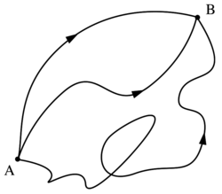 在时间t0,粒子从点A出发,则在时间t1,可能出现在点B。图中的三条路径,皆对此量子幅有贡献。(也有许多其他路径。)
量子力学中,哈密顿算符 生成时间演化算符
 :
:

一个量子粒子在时刻 到
到 间从位置
间从位置 运动到
运动到 的量子概率幅是:

因为是很复杂的算符函数,直接用以上定义计算 非常困难。
非常困难。
时间演化算符符合

因此量子幅符合
 。
。
右式被积项的意义为从 出发,在中途时刻
 先穿过位置
先穿过位置 ,再到达
,再到达 的路径的总量子幅,此量子幅是两段路径量子幅的积;而左式从到的量子幅,等于右式所有这种路径的和(积分)。
假设粒子在时刻到间从位置运动到。那可以把之间的时间平均分割成个别的时间区间: 。每一段的时间是
 。
在时刻
。
在时刻 和
和 间粒子的量子幅是:

因为 和
和 是互不交换的算符,所以必须运用它们的交换子关系:
![{\displaystyle [{\hat {p}},{\hat {x}}]=i\hbar }](https://wikimedia.org/api/rest_v1/media/math/render/svg/43820e23757c344301c3c65299b2c455d09321f1) 把
把 修成所有的在左方的正常顺序:

做时间切片的作用是:当取切片数趋向无限大的极限时( ),原本非正常顺序的哈密顿算符可以以正常顺序版代替。在正常顺序算符下,和从算符简化成普通复数。
因此
),原本非正常顺序的哈密顿算符可以以正常顺序版代替。在正常顺序算符下,和从算符简化成普通复数。
因此

把所有连接和的路径相加得到的总量子幅是:
![{\displaystyle {\begin{aligned}iG(x_{b},t_{b};x_{a},t_{a})&=\int dx_{1}\cdots dx_{n-1}\prod _{i=1}^{n-1}dp_{i}\exp \left[{\frac {i}{\hbar }}\sum _{j=1}^{n-1}\Delta \,L\left(t_{j},{\frac {x_{j}+x_{j-1}}{2}},{\frac {x_{j}-x_{j-1}}{\Delta }}\right)\right]\\&=\int {\mathcal {D}}\left[x(t)\right]e^{{\frac {i}{\hbar }}S[x(t)]},\end{aligned}}}](https://wikimedia.org/api/rest_v1/media/math/render/svg/dbe906f20c437e6755b35f4f5f9aacc530cc995c)
其中 是路径
是路径 的作用量,拉格朗日量
 的时间积分:

自由粒子的作用量( ,
, )为:
)为:

可以插入路径积分里做直接计算。
暂时把指数函数内i去掉可容许比较简易的理解计算,以后可以用威克转动回到原式。去掉 后,有:
后,有:

其中 是以上时间切成有限片的积分。连乘里,每一项都是平均值为,方差为
 的高斯函数。故多重积分是相邻时间高斯函数
 的卷积:
的卷积:

这里面共包含 个卷积。傅里叶变换下,卷积变成普通乘积:

而高斯函数的傅里叶变换也是一个高斯函数:

因此

反傅里叶变换可以得到实空间量子幅:

时间切片方法原则上不能决定以上比例系数,但以随机运动概率来理解,可得到以下正规条件:

从这条件可得到扩散方程:

回到振荡轨道,即恢复分子里的原本的。这可同样得到一系列高斯函数的卷积。但这些高斯积分是严重振荡积分而要小心计算。一个普遍方法是让时间片带一个小虚部。这等同于以威克转动在实时间和虚时间间转换。在这些处理下,可得到传播核:

运用和之前一样的正规条件,重新得到自由粒子的薛定谔方程:

这意味着任何 的线性组合也符合薛定谔方程,包括以下定义的波函数:

和一样服从薛定谔方程:

配分函数成为泛函积分:

费米积分、格拉斯曼数


 . PMID 16577107. doi:10.1073/pnas.14.2.178.
